
The independent sample t-test is a parametric test specifically used to compare the means of two independent groups and determine whether there is statistical evidence of significant differences in their associated population means. The variables involved when performing an independent sample t-test are identified as dependent variables and independent/grouping variables.
The independent sample t test is alternatively referred to as:
- Independent t-test
- Independent Measures t-test
- Independent Two-sample t-test
- Student t-test
- Two-Sample t-test
- Uncorrelated Scores t-test
- Unpaired t-test
- Unrelated t-test
When is Independent Sample T Test Used?
The Independent Samples t-test is mainly used to test whether:
- There is a significant mean difference between the two groups
- There is a significant mean difference between the two independent interventions
- There is a significant mean difference between two scores (eg, whether there is a difference in performance between math and science exams).
Please note that the Independent Samples t-test is limited to comparing means for only two groups. It cannot be used to make comparisons among more than two groups. If you need to compare means across more than two groups, running an ANOVA is likely the appropriate method.
You can also check out our tutorials on how to perform a one-way ANOVA in SPSS and how to report one-way ANOVA SPSS output in APA format.
Assumptions of Independent Sample T-Test
Your data must satisfy the following criteria for conducting the Independent Samples t Test:
- The dependent variable must be continuous, at the interval or ratio level.
- Independent variables must be categorical with exactly two categories.
- Cases should have values on both the dependent and independent variables.
- Samples/groups must be independent, meaning there should be no relationship between the subjects in each sample: a. Subjects in the first group cannot overlap with those in the second group. b. No subject in either group can influence subjects in the other group. c. Neither group can influence the other group. Violating this assumption will lead to inaccurate p-values.
- A random sample of data should be taken from the population.
- The dependent variable should have a normal distribution (approximately) within each group. Non-normal population distributions, especially those with thick-tailed or heavily skewed data, can substantially reduce the test’s power. However, in moderate or large samples, a violation of normality may still yield accurate p-values.
- Homogeneity of variances is necessary, meaning variances should be approximately equal across groups. a. When this assumption is violated and sample sizes for each group differ, the p-value is not reliable. b. The Independent Samples t Test output also includes an approximate t statistic (Welch t Test statistic) that does not assume equal population variances. This statistic can be used when equal variances among populations cannot be assumed, and it is also known as the Unequal Variance t-test or Separate Variances t-test.
- No outliers should be present in the data.
In cases where one or more assumptions for the Independent Samples t-test are not met, researchers may consider using the nonparametric Mann-Whitney U Test instead.
Hypotheses in Independent Sample T Test
The null hypothesis (H0) and alternative hypothesis (H1) of the Independent Sample t-test can be expressed in two different but equivalent ways:
H0: µ1 = µ2 (“the two population means are equal”)
H1: µ1 ≠ µ2 (“the two population means are not equal”)
OR
H0: µ1 – µ2 = 0 (“the difference between the two population means is equal to 0”)
H1: µ1 – µ2 ≠ 0 (“the difference between the two population means is not 0”)
where µ1 and µ2 are the population means for group 1 and group 2, respectively.
Understanding the Levene’s Test for Equality of Variances in Independent t test
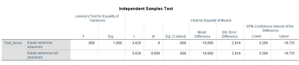
In the context of the Independent Sample t-test, it is essential to assume homogeneity of variance, meaning both groups should have the same variance. To conveniently assess this assumption, SPSS includes Levene’s Test, which evaluates the equality of variances, whenever you run an independent sample t-test.
The hypotheses for Levene’s test are:
- H0: σ12 – σ22 = 0 (“the population variances of group 1 and 2 are equal”)
- H1: σ12 – σ22 ≠ 0 (“the population variances of group 1 and 2 are not equal”)
Rejecting the null hypothesis of Levene’s Test implies that the variances of the two groups are not equal, indicating a violation of the homogeneity of variances assumption.
In the Independent Sample Test table, you will find two rows of output: “Equal variances assumed” and “Equal variances not assumed.” Depending on the outcome of Levene’s test (i.e., large p-value for equal variances, or small p-value for unequal variances), you will choose the appropriate row of output to interpret the results of the actual Independent Sample t Test (under the heading “t-test for Equality of Means”).
When equal variances are assumed (large p-value), the calculation of the independent sample t-test statistic uses pooled variances. On the other hand, when equal variances cannot be assumed (small p-value), the calculation utilizes un-pooled variances along with a correction to the degrees of freedom. This distinction in the calculation accounts for the potential differences in variances between the two groups and ensures the accuracy of the test results.
tential differences in variances between the two groups and ensures the accuracy of the test results.
Test Statistic in Independent Sample T Test
The Independent Samples t-test employs a test statistic denoted as “t,” which has two forms, depending on whether equal variances are assumed or not. SPSS generates both forms to cater to different scenarios, and both are described below. It is important to note that the null and alternative hypotheses remain identical for both forms of the test statistic.
EQUAL VARIANCES ASSUMED (Homogeneity of Variance Assumed)
When we assume that the two independent samples are drawn from populations with equal variances (homogeneity of variance assumed), the test statistic “t” is calculated as follows:

where:
x̄1 is the mean of the first sample
x̄2 is the mean of the second sample
n1 is the sample size (number of observations) of the first sample
n2 is the sample size (number of observations) of the second sample
sp is the pooled standard deviation calculated as

where:
s12 is the sample variance of the first sample
s22 is the sample variance of the second sample
The calculated “t” value is then compared to the critical t value from the t-distribution table with:
Degrees of freedom (df) = n1 + n2 – 2 and the chosen confidence level.
That is, the critical value is obtained from t tables using the following formula:
tα/2, n1+n2-2, For a two-tailed t-test
tα, n1+n2-2, For a one-tailed t-test
If the calculated “t” value is greater than the critical t value, we reject the null hypothesis.
Note: This form of the independent samples t-test statistic assumes equal variances. The assumption allows us to “pool” the sample variances (sp). However, if this assumption is violated, the pooled variance estimate may not be accurate, which can affect the precision of our test statistic (and consequently, the p-value). In this case, we conduct a different t-test that assumes unequal variance. This type of t-test is widely known as the Welch’s t-test.
EQUAL VARIANCES NOT ASSUMED (Homogeneity of variance assumption violated)
When we assume that the two independent samples are drawn from populations with unequal variances (homogeneity of variance assumption violated), the test statistic “t” is computed as follows:

where:
x̄1 is the mean of the first sample
x̄2 is the mean of the second sample
n1 is the sample size (number of observations) of the first sample
n2 is the sample size (number of observations) of the second sample
s1 is the standard deviation of the first sample
s2 is the standard deviation of the second sample
The calculated “t” value is then compared to the critical t value from the t-distribution table with degrees of freedom (df) calculated as:

and the chosen confidence level. If the calculated “t” value is greater than the critical t value, we reject the null hypothesis.
Note: This form of the independent samples t-test statistic does not assume equal variances. As a result, both the denominator of the test statistic and the degrees of freedom for the critical t value are different from the equal variances form of the test statistic.
How to Run an Independent Sample T-Test In SPSS
Independent T-Test Example
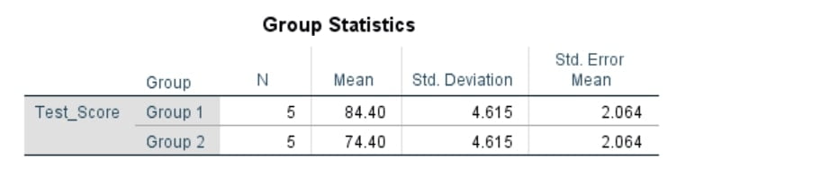
A school principal wants to determine if there is a significant difference in the test scores of students who participated in an after-school tutoring program compared to those who did not. The test scores are collected from two groups of students: those who attended the tutoring program (Group 1) and those who did not (Group 2). The principal aims to use an independent samples t-test to analyze the data.
The Independent T-Test Sample Dataset can be downloaded below;
Research Question: Is there a significant difference in the average test scores between students who participated in the after-school tutoring program and those who did not?
Hypotheses:
- Null Hypothesis (H0): There is no significant difference in the average test scores between the two groups.
- Alternative Hypothesis (H1): There is a significant difference in the average test scores between the two groups.
Performing Independent Sample T-Test In SPSS: Test Procedure
If you want to perform an independent sample T-test using SPSS, you only need to import the data into SPSS and simply follow these quick steps:
Performing an independent sample T-Test in SPSS is as simple as ABC. Just follow the following 4 steps:
- Step 1: From the Main Menu, Click Analyze > Compare Means > Independent-Samples T-Test.

The “Independent-Samples T Test” dialog box will appear as shown below:

- Step 2: Select (Test_Score) as the test variable and move it to the Test Variable(s) list.
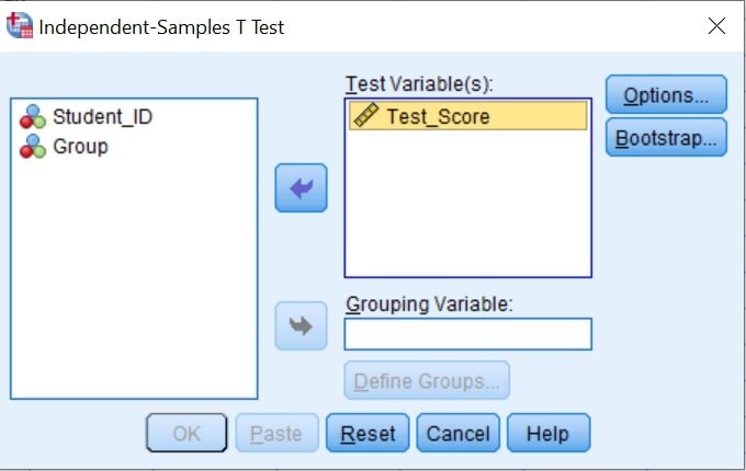
Note. If you have two or more test variables (dependent variables), you need to transfer all of them to the Test Variable (s) box. In such a case, a separate t-test is computed for each variable.
- Step 3: Select a single grouping variable (Group) and move it to the Grouping Variable box.
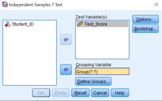
- Step 4: Click Define Groups to specify the two codes that identify your two groups.
In our case, Group 1 was coded as 1 and Group 2 was coded as 2. So, you need to define them as shown below;
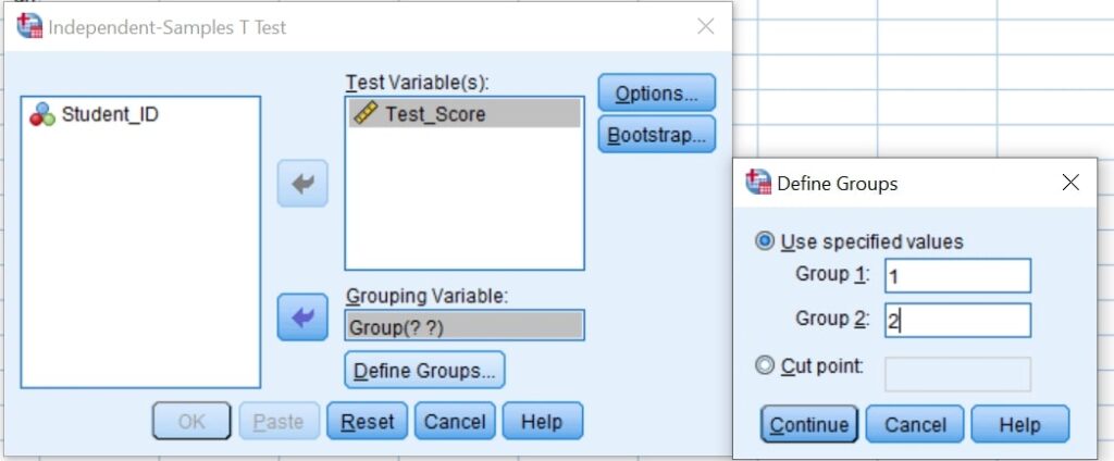
Note. If you coded the groups as 0 and 1, you should specify the same in Group 1 and Group 2 boxes.
- Step 6: Click Continue.
- Step 7: Click OK.
The Independent Sample T-Test SPSS Outputs Will be displayed as shown below;
Unsure how to interpret and report your independent samples t-test results in APA format? Master the process with our in-depth guide on interpreting Independent Sample T-Test SPSS Outputs.