Performing Pearson’s Correlation Using SPSS

Pearson’s correlation coefficient is a widely used statistical test. It primarily determines the strength and direction of the linear relationship between two continuous variables. This article provides an overview of Pearson’s correlation analysis, its assumptions, how to run Pearson’s correlation in SPSS, and how to interpret Pearson’s Correlation SPSS Outputs.

Quick Steps

1. From the SPSS Main Menu, Click Analyze –> Correlate –> Bivariate
2. Transfer the variables Hours_studied and Exam_score into the Variables: box.
3. Make sure the Pearson is Checked under Correlation Coefficient
4. Click OK.

What is Pearson’s Correlation?

Pearson’s correlation coefficient also known as Pearson Correlation is a parametric statistical test that is used to determine the strength and direction of a linear relationship between two continuous variables. Pearson’s correlation coefficient value generally lies between -1 and +1, with values closer to 1 indicating strong relationship and those close to 0 indicating weak relationships.

Below is a summary of how to determine the strength and direction of linear relationships based on Pearson’s correlation coefficient values:

Strength of relationship	Positive Correlation	Negative Correlation
Zero	0	0
Weak	0.1 to 0.3	-0.1 to -0.3
Moderate	0.3 to 0.7	-0.3 to -0.7
Strong	0.7 to 1.0	-0.7 to -1.0
Perfect	1	-1

Correlation can be categorized into 3:

• Positive Correlation – The correlation coefficient value is positive. This suggests that as one variable increases, the other variable also tends to increase.
• Negative Correlation – The correlation coefficient value is negative. This suggests that as one variable increases, the other variable tends to decrease.
• No Correlation – The correlation coefficient value is 0. This suggests that there is no linear relationship between the two variables.

Pearson’s Correlation Assumptions

Before you start performing Pearson’s correlation analysis in SPSS, it is always advisable to confirm whether the assumptions are met. The main assumptions include:

Assumption #1: The two Variables should be Continuous

The two variables should be measured on a continuous scale (they should be measured at the interval or ratio level).  Examples of continuous variables are, exam scores measured as a percentage and the number of hours spent studying.

Assumption #2: Linear Relationship

There should be a linear relationship between the two variables. This assumption can be checked using SPSS by creating a scatterplot. The scatterplot can resemble one of these:  

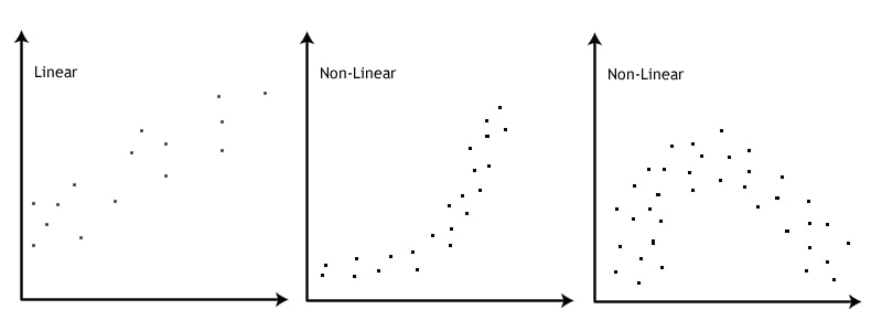
If after creating a scatterplot there is a non-linear relationship, then you need to use a non-parametric equivalent of Pearson’s Correlation Coefficient. Specifically, you’ll need to run a Spearman’s Correlation instead. Alternatively, you can consider transforming your variables to see if there is a linear relationship between the transformed variables.

Assumption #3: No Significant Outliers

There should be no significant outliers. An outlier is a single observation that lies far away from other data points. Pearson’s correlation coefficient is highly influenced by outliers. Thus, it is necessary to remove any significant outlier before running Pearson’s correlation in SPSS. The figure below demonstrates the effects of outliers on Pearson’s correlation coefficient value.

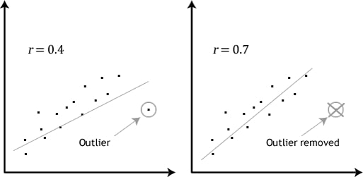
The figure above shows that Pearson’s correlation coefficient, r, is highly influenced by outliers. In other words, Pearson’s correlation coefficient is sensitive to outliers and this can have significant effects on the line of best fit. Specifically, a scatter plot with an outlier yielded a correlation coefficient value of 0.4. However, when the outlier is removed, the coefficient increases to 0.7. Therefore, it is necessary to examine whether there are significant outliers before performing Pearson’s correlation in SPSS.

Assumption #4: Normality

The data for the variables should be approximately normally distributed. This assumption can be performed using the Shapiro-Wilk Test or the Kolmogorov-Smirnov test. You can check our detailed guide on how to run normality tests in SPSS.

Note. If the above assumptions are not met, then performing a Pearson’s correlation will yield invalid and unreliable results.

How to Perform Pearson’s Correlation in SPSS

Example Pearson’s Correlation Test

The university wants to understand how study habits affect academic performance. Specifically, they aim to determine whether the number of hours students study per week correlates with their final exam scores. To explore this, they collected data from 30 students, asking each one to report the number of hours they studied per week along with their final exam scores. The data obtained were as shown below:

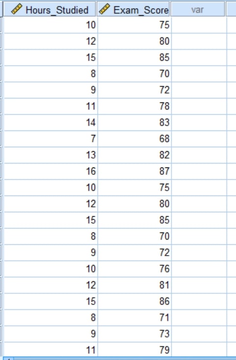
The complete dataset can be downloaded below.

The above data is in Excel format (.xlsx). Check out our detailed guide on how to import Excel data into SPSS.

Pearson’s Correlation in SPSS: Test Procedure

To run a Pearson’s correlation analysis in SPSS, just follow these 4 simple steps:

• Step 1. From the SPSS Main Menu, Click Analyze –> Correlate –> Bivariate

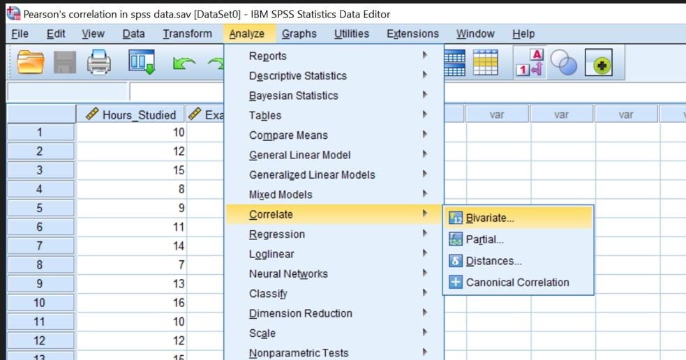
You will be presented with the following bivariate dialog box

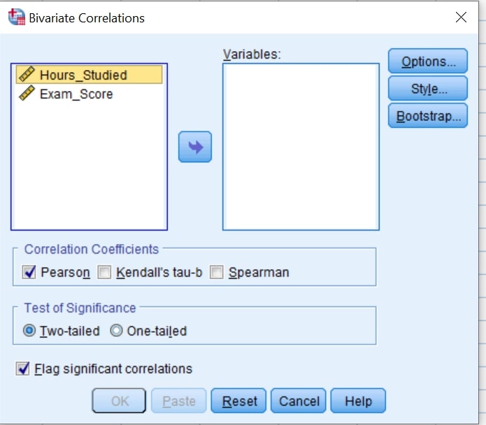
• Step 2. Transfer the variables Hours_studied and Exam_score into the Variables: box. This can be done either by dragging and dropping them or by clicking on them and then clicking on the arrow button pointing to the Variables: box.

You should have a similar screen display as shown below;

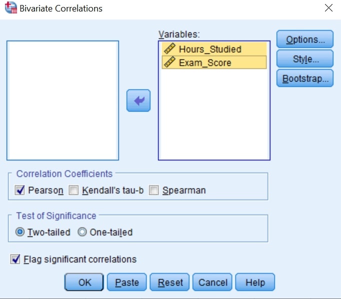
• Step 3: Make sure the Pearson is Checked under Correlation Coefficient
• Step 4: Click OK.

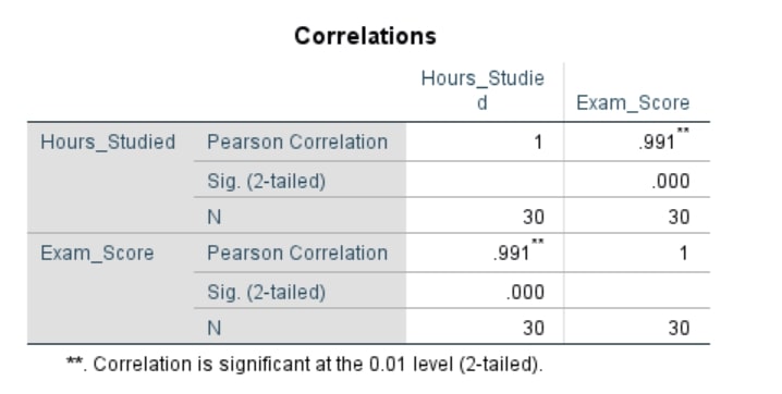
You’ll have the Pearson’s Correlation SPSS Outputs as shown below;