Reporting Pearson’s Correlation Analysis in SPSS [Perform, Interpret & Report]

Pearson’s correlation is a statistical measure used to assess the strength and direction of a linear relationship between two variables. It is widely used in research and data analysis to understand how one variable changes in relation to another. In this article, we will guide you on how to interpret and report Pearson’s correlation outputs from SPSS. Clear and accurate reporting of these results is essential, especially in academic and professional contexts. Properly presenting your findings helps ensure that your conclusions are understandable and credible. By following this guide, you will learn how to present your SPSS outputs effectively and avoid common mistakes.

What is Pearson’s Correlation?

Pearson’s correlation, usually denoted by a Greek letter “ρ”, or “r” is a statistical test that measures the strength and direction of a linear relationship between two continuous variables. Let’s consider a scenario where you’ve plotted your data using a Scatter Plot and the points tend to form a straight diagonal line (either upwards, or downwards). In such a case, it is worth running a Pearson’s correlation analysis to quantify the strength of the linear relationship.

It is worth noting that:

• A positive correlation (r between 0 and 1) indicates that as the value of one variable increases, the other variable tends to increase as well.
• A negative correlation (r between -1 and 0) means that as one variable goes up, the other tends to go down.
• A correlation close to zero suggests little to no linear relationship between the variables.

NOTE: Correlation value does not imply causation! Just because two things are correlated doesn’t mean one variable causes the other. There might be a third unseen factor influencing both variables.

Assumptions of Pearson’s Correlation

While Pearson’s correlation is a powerful statistical test, its reliability and validity depend on several assumptions: Some of these assumptions include:

1. Continuous Variables: The two variables under investigation must be measured on a continuous scale (either interval or ratio measure). Some examples of continuous variables include; height, weight, or exam scores.
2. Linear Relationship: The correlation coefficient measures the strength of a linear relationship between two variables. This means that it is not ideal for non-linear relationships.
3. Normally Distributed Data: Ideally, the data for both variables should be approximately normally distributed.

If your data doesn’t meet these assumptions, alternative correlation measures such as Spearman’s Correlation might be more suitable.

Recall: Checking these assumptions before interpreting your Pearson’s correlation results ensures you’re drawing reliable conclusions from your data.

Steps to Perform Pearson’s Correlation in SPSS: Quick Guide

To perform Pearson’s correlation in SPSS, follow these steps:

1. Prepare your dataset to ensure it’s suitable for Pearson’s correlation.
2. Open SPSS and load your dataset.
3. Navigate to Analyze > Correlate > Bivariate.
4. Select the variables you want to analyze.
5. Choose Pearson as the correlation type.
6. Decide whether to use a two-tailed or one-tailed test based on your hypothesis.
7. Click OK to generate the output.

Still struggling with the above quick guide? Check out our complete guide on how to perform Pearson’s correlation analysis in SPSS for more details.

Understanding SPSS Outputs for Pearson’s Correlation

Now that you’ve learned how to run Pearson’s correlation analysis in SPSS (refer to this guide for example used and how to perform the test using SPSS) in our previous guide, let’s dive into interpreting the Pearson’s Correlation SPSS outputs.

Correlation Table

The correlation table in SPSS provides several key pieces of information:

• Variables: Lists the two variables being analyzed.
• Correlation Coefficients: The Pearson correlation coefficient (r), indicates the strength and direction of the relationship between the variables.
  • Weak correlation: r between 0.1 and 0.3 (positive or negative).
  • Moderate correlation: r between 0.3 and 0.7 (positive or negative).
  • Strong correlation: r between 0.7 and 1 (positive or negative).
• Significance Values (p-value): Indicates whether the correlation is statistically significant.
• Sample Size: The number of pairs of data points used in the analysis.

Example Pearson’s Correlation SPSS Table

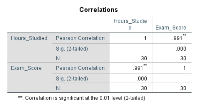
From the above SPSS table:

• The variables are: hours studies and exam score
• The Pearson’s correlation coefficient is 0.991. This value is positive and very close to 1 (hence strong positive correlation)
• The p-value is denoted by sig. (2-tailed) = 0.000
• The sample size, denoted by N is 30

Interpretation of Pearson’s Correlation SPSS Results

Based on the above outputs;

• Pearson Correlation: The correlation coefficient (r) between hours studied and exam scores is .991, which is very close to 1. This indicates that there was a very strong positive relationship between these two variables.
• Significance (2-tailed): The p-value is .000, which is less than .001. This indicates that the correlation is statistically significant at the 0.01 level of significance.
• N: The sample size (n) is 30 for both variables.

Reporting Pearson’s Correlation Analysis Results

When reporting Pearson’s correlation results, it is important to follow a clear and structured format. Here’s a general structure:

1. Statement of the test conducted:
   • Mention that you performed a Pearson correlation analysis to assess the relationship between the two variables.
2. Key results:
   • Include the correlation coefficient (r), the sample size (N), and the p-value.
   • Example: “The Pearson correlation between hours studies and exam score was r = 0.991, based on 30 participants, and the result was statistically significant, p = 0.000.”
3. Contextual interpretation of results:
   • Explain what the correlation means in the context of your research.
   • Example: “This suggests a strong positive relationship between hours studied and exam scores, meaning that as hours studied increases, exam scores tend to increase as well.”

APA Style Example

A Pearson correlation analysis was conducted to examine the relationship between the number of hours studied per week and the final exam scores among university students. The results indicated a very strong, positive, and significant correlation between hours studied and exam scores, r(28)=.991, p<.001. This result indicates that as the number of hours studied per week increases, the final exam scores also tend to increase significantly. In other words, the finding suggests that higher numbers of study hours are associated with higher exam scores.

Conclusion

Properly interpreting and reporting Pearson’s correlation outputs is crucial for presenting accurate and meaningful results. Clear reporting ensures that your findings are easily understood and trusted by your audience, whether in academic research or professional analysis. By following best practices and providing a clear interpretation of the correlation coefficient and significance, you enhance the quality of your analysis.

We encourage you to always follow these steps for clear and accurate reporting of Pearson’s correlation results. However, if you need further assistance or have any questions regarding SPSS analysis, feel free to reach out. Our team is here to help you with your SPSS data analysis needs.